Subtle pitfalls of conditional probabilities and the Borel-Kolmogorov paradox
TL;DR
I’m aggregating the stuff I have learned while teaching ML and SLT classes at the ETH — about subtleties of defining the notions of conditional probabilities and expectations. Will cover the problem of defining $P(Y \vert X = x)$ in case of $P(X = x) = 0$, describe the Borel-Kolmogorov paradox and give its intuitive explanation.
It is not that easy.
Contents
Outline
Intro
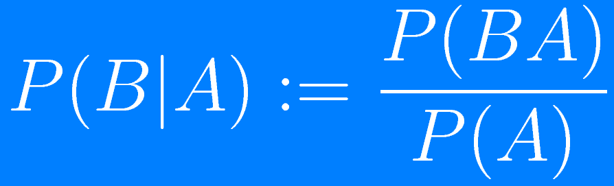
Although simple at first glance, the notions of conditional probability and conditional expected value are not that simple. To start with, the conventional definition of conditional probability in “classical” probability theory
$$ \begin{equation} P(B \vert A) = \frac{P(B \cap A)}{P(A)} \label{eq:prob} \end{equation} $$
turns out to be ill-formed in some cases (discussed below). To continue, the conditional expected value is not a value (i.e. it is not a number at all, as you would naturally expect an expectation to be, excuse my pun1), but rather a random variable (this is the second point to recap below).
Since this is something both interesting for beginners to dig into and to for advanced learners think about, I decided to make an attempt to systematize, relearn it myself and share.
While conditional probabilities are covered in this post, I’ll tackle conditional expectations in the next one (time permitting :-)).
A simple example highlighting the problem
The simple equation \eqref{eq:prob} above is the right definition when it is assumed that the event $A$ has a non-zero probability measure: $P(A) > 0$. But what if this assumption doesn’t hold? Is all ruined then?
Let’s describe a simple example situation, where $P(Y \vert X = x)$ does intuitively make sense, however, it is undefined according to the definitions above which make use of the division by $P(X = x)$.
Consider a random variable $X \sim U([0, 1])$2. For each value of $X$, another random variable $Y$ is the result of a coin toss, where
If we, in an attempt to define the conditional probability of the event, say, $P(Y = \text{“heads”} \vert X = x)$, take the path similar to \eqref{eq:prob}, it will be undefined since $P(X = x) = 0$ everywhere on $[0, 1]$.
However, intuitively (just from looking into how $Y$ is defined), the conditional probability should be
First attempt to overcome the issue
The issue highlighted above (zero-measure events) can be addressed in the following way: remember that although the event ${X = x}$ above has zero measure3, it has a nonzero density $ p(x) = 1 $ for all $x \in [0, 1]$.
This leads to the idea of defining conditional density rather than conditional probability:
This yields “kind of” a correct result and, in fact, one can see such a definition in most textbooks on stats/prob… however, there’s still a problem. It is highlighted by the so called Borel-Kolmogorov paradox.
The issue persists: Borel-Kolmogorov paradox
In essence, it turns out that our stubborn attempts to define anything w.r.t. to a point event of measure zero is ill-formed without considering some more context (what “context” means will be clear in a minute).
Consider4 a unit sphere in $$\mathbb{R}^3$$ on which we have constructed a uniform distribution in the following way5:
First, we sample the longitude angle (a.k.a. “angle along the equator”) $\lambda \in [-\pi, \pi]$ uniformly at random:
$$ \lambda \sim p(\lambda) = \frac{1}{2\pi}. $$Second, we sample the latitude angle (a.k.a. “angle along the meridian”) $\varphi \in [-\pi/2, \pi/2]$ with density:
$$ \varphi \sim p(\varphi) = \frac{1}{2} \cos \varphi. $$
Once again5, at this point I encourage you to either just believe or check out the post in the footnote, that this procedure produces a uniform distribution on the sphere.
We are now going to build the “paradox” by computing the conditional probability densities \eqref{eq:cond} on two of the so called great circles:
- on the equator and 2) on the meridian.
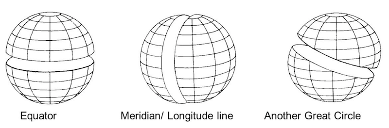
Credit of the image to https://slideplayer.com/slide/9119414/
The joint distribution apparently has the density
$$ p(\lambda, \varphi) = \frac{1}{4\pi} \cos \varphi. $$
Let us compute the conditional density on the equator (i.e. $\varphi = 0$):
$$ \begin{equation}\label{eq:phi-zero} p(\lambda \vert \varphi = 0) = \frac{\left. p(\lambda, \varphi) \right\vert_{\varphi=0}} {\left. p(\varphi) \right\vert_{\varphi=0}} = \frac{1}{2\pi}, \end{equation} $$
which happens to be uniform as expected. But the second one — the conditional density on the meridian (i.e. $\lambda = 0$) — turns out to be non-uniform:
$$ \begin{equation}\label{eq:lambda-zero} p(\varphi \vert \lambda = 0) = \frac{\left. p(\lambda, \varphi) \right\vert_{\lambda=0}} {\left. p(\lambda) \right\vert_{\lambda=0}} = \frac{1}{2} \cos \varphi. \end{equation} $$
Amazing, isn’t it? Uniform sphere, all is symmetric, we take two equivalent great circles which must be just an orthogonal6 coordinate transform of each other — and get two completely different results.
This is a rare case when one needs to understand what is being done. As E. T. Jaynes wrote,
For the most part, the transition from discrete to continuous probabilities is uneventful, proceeding in the obvious way with no surprises. However, there is one tricky point concerning continuous densities that is not at all obvious, but can lead to erroneous calculations unless we understand it. The following example continues to trap many unwary minds.
E.T. Jaynes, “Probability Theory: the Logic of Science”
So let’s move on to a short explanation.
The reason behind the Borel-Kolmogorov paradox
What we did so far was:
- We identified the problem: one can’t perform the division by zero when conditioning on the event of measure zero.
- We then tried to solve this issue by transitioning from the ratio of probabilities to the ratio of probability densities, hoping that this would solve the issue of the division by zero.
However, the ratio of densities is a tricky object, and we will now explain why. It always requires the limiting procedure to be specified7. Although each of the densities involved in our story is alone well-defined regardless of the limiting procedure, the ratios of these densities can behave differently depending on which events compose the limiting family of events.
In other words, for a point event $A = {X = x}$ we have to specify how to construct the sequence of enclosing events
I’d like to stress it:
Failing to specify the limiting procedure is the reason that leads to the Borel-Kolmogorov paradox.
Let’s formalize and visualize it a bit.
First, consider the computation of $p(\lambda \vert \varphi = 0)$ (eq. \eqref{eq:phi-zero} above): if we expand the limit definitions of the densities involved, we get (note a slight abuse of notation here8)
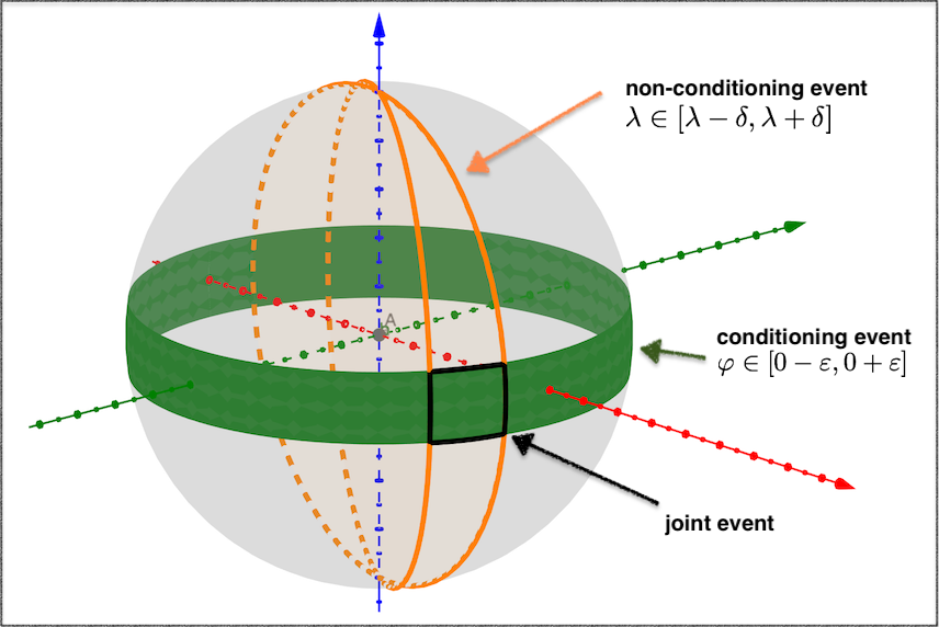
Visualization of defining the limiting ratio of $p(\lambda \vert \varphi = 0)$. The shape of the family of conditioning events (green), yields uniform ratio regardless of longitude.
The green area denotes the denominator (i.e. conditioning) event $\varphi \in [0-\varepsilon, 0 + \varepsilon]$, and the orange section denotes the event on the non-conditioning variable, i.e. $\lambda \in [\lambda - \delta, \lambda + \delta]$. The black spherical polygon is the joint event.
Second, for the computation of $p(\varphi \vert \lambda = 0)$ (eq. \eqref{eq:lambda-zero} above) we get (again, with the notation abuse8)
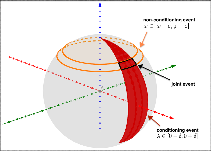
Visualization of defining the limiting ratio of $p(\varphi \vert \lambda = 0)$. The shape of the family of conditioning events (red), yields a non-uniform ratio which depends on the latitude.
Now the variables are swapped compared to the previous case. The red area denotes the denominator (i.e. conditioning) event $\lambda \in [0-\delta, 0 + \delta]$, and the orange section denotes the event on the non-conditioning variable $\varphi$, i.e. $\varphi \in [\varphi - \varepsilon, \varphi + \varepsilon]$. As previously, the black spherical polygon is the joint event.
What do the two ways of computing $p(\cdot \vert \cdot)$ have in common? In both cases, we compute the limiting ratio of the area inside the black rectangle (joint event) to the colored area (conditioning event).
But what makes the two cases different? From the visualization above one can see that:
- In the former case, regardless of the longitude (choice of $\lambda$), the joint events would always occupy the same fraction of the conditioning events — due to the “parallel-sliced” shape of the sequence of conditioning events.
- In the latter case, the fraction occupied by the joint events w.r.t to the conditioning events depends on the latitude (choice of $\varphi$) due to a specific “angular-sliced” shape of the sequence of conditioning events.
That’s it. The above actually explains what happens inside limits - the probability ratio of the two families of limiting events behaves differently depending on the choice of these families.
As an exercise, one can try inventing even more weird limiting families that yield more complex conditional density formulae than those of \eqref{eq:phi-zero}, \eqref{eq:lambda-zero}.
What’s next?
In the next part, I’ll try to describe the way mathematicians deal with the above paradox — namely via conditional expectations with respect to $\sigma$-algebras.
References
- Yarin Gal, Talk on the Borel-Kolmogorov paradox
- E.T. Jaynes, “Probability Theory: the Logic of Science”, Ch. 15
Notes
Since we are at puns, here is just a funny image on it. ↩︎
$X \sim U([0, 1])$ denotes a uniform distribution over the support of $[0, 1]$. ↩︎
A propos, for a slightly more advanced reader: convince yourself that that the event ${X = x}$ belongs to a Borel $\sigma$-algebra of $[0, 1]$, an hence is measurable. ↩︎
I elaborate here on the talk by Yarin Gal on Borel-Kolmogorov paradox. ↩︎
A naïve strategy of generating a uniform point on the unit sphere by just uniformly sampling a longitude angle from $[-\pi, \pi]$ and then uniformly sampling a latitude angle from $[-\pi/2, \pi/2]$ is in fact incorrect. The intuitive reason lies in the fact that uniformly sampled latitude yields more condense points around the north and south poles, since the surface is, informally speaking, “glued together” there.\ For more, check out this explanation. ↩︎ ↩︎
Preserves distances, an hence — volumes. ↩︎
Probability density, by one of its definitions, is the derivative of cumulative distribution function. ↩︎
In order to possibly keep things simple, we terribly abuse the notation and write $P(\lambda \pm \delta, \varphi \pm \varepsilon)$ to denote the joint probability of range events $\lambda \in [\lambda - \delta, \lambda + \delta]$ and $\varphi \in [\varphi - \varepsilon, \varphi + \varepsilon]$ ↩︎ ↩︎
Want to discuss anything? Comments are welcome via e-mail alexey@gronskiy.com, Telegram @agronskiy or any other social media.